Imager¶

class oskar.Imager(precision=None, settings=None)¶

This class provides a Python interface to the OSKAR imager.

The oskar.Imager class allows basic (dirty) images to be made from simulated visibility data, either from data files on disk, from numpy arrays in memory, or from oskar.VisBlock objects.

There are three stages required to make an image:

Create and set-up an imager.
Update the imager with visibility data, possibly multiple times.
Finalise the imager to generate the image.

The last two stages can be combined for ease of use if required, simply by calling the run() method with no arguments.

To set up the imager from Python, create an instance of the class and set the imaging options using a oskar.SettingsTree created for the oskar_imager application, and/or set properties on the class itself. These include:

algorithm and weighting
cellsize_arcsec or fov_deg
channel_snapshots
fft_on_gpu and grid_on_gpu
image_size
image_type

To optionally filter the input visibility data, use:

freq_max_hz and freq_min_hz to exclude visibilities based on frequency.
time_max_utc and time_min_utc to exclude visibilities based on time.
uv_filter_max and uv_filter_min to exclude visibilities based on their (u,v)-baseline length in wavelengths.

To specify input and/or output files, use input_file and output_root.

For convenience, the set() method can be used to set multiple properties at once using kwargs.

Off-phase-centre imaging is supported. Use the set_direction() method to centre the image around different coordinates if required.

When imaging visibility data from a file, it is sufficient simply to call the run() method with no arguments. However, it is often necessary to process visibility data prior to imaging it (perhaps by subtracting model visibilities), and for this reason it may be more useful to pass the visibility data to the imager explicitly either via parameters to run() (which will also finalise the image) or using the update() method (which may be called multiple times if necessary). The convenience method update_from_block() can be used instead if visibility data are contained within a oskar.VisBlock.

If passing numpy arrays to run() or update(), be sure to set the frequency and phase centre first using set_vis_frequency() and set_vis_phase_centre().

After all visibilities have been processed using update() or update_from_block(), call finalise() to generate the image. The images and/or gridded visibilities can be returned directly to Python as numpy arrays if required.

Note that uniform weighting requires all visibility coordinates to be known in advance. To allow for this, set the coords_only property to True to switch the imager into a “coordinates-only” mode before calling update(). Once all the coordinates have been read, set coords_only to False, initialise the imager by calling check_init() and then call update() again. (This is done automatically if using run() instead.)

Examples

>>> # Generate some data to process.
>>> import numpy
>>> n = 100000  # Number of visibility points.
>>> # This will generate a filled circular aperture.
>>> t = 2 * numpy.pi * numpy.random.random(n)
>>> r = 50e3 * numpy.sqrt(numpy.random.random(n))
>>> uu = r * numpy.cos(t)
>>> vv = r * numpy.sin(t)
>>> ww = numpy.zeros_like(uu)
>>> vis = numpy.ones(n, dtype='c16')  # Point source at phase centre.

To make an image using supplied (u,v,w) coordinates and visibilities, and return the image to Python:

>>> # (continued from previous section)
>>> imager = oskar.Imager()
>>> imager.fov_deg = 0.1             # 0.1 degrees across.
>>> imager.image_size = 256          # 256 pixels across.
>>> imager.set_vis_frequency(100e6)  # 100 MHz, single channel data.
>>> imager.update(uu, vv, ww, vis)
>>> data = imager.finalise(return_images=1)
>>> image = data['images'][0]

To plot the image using matplotlib:

>>> # (continued from previous section)
>>> import matplotlib.pyplot as plt
>>> plt.imshow(image)
>>> plt.show()

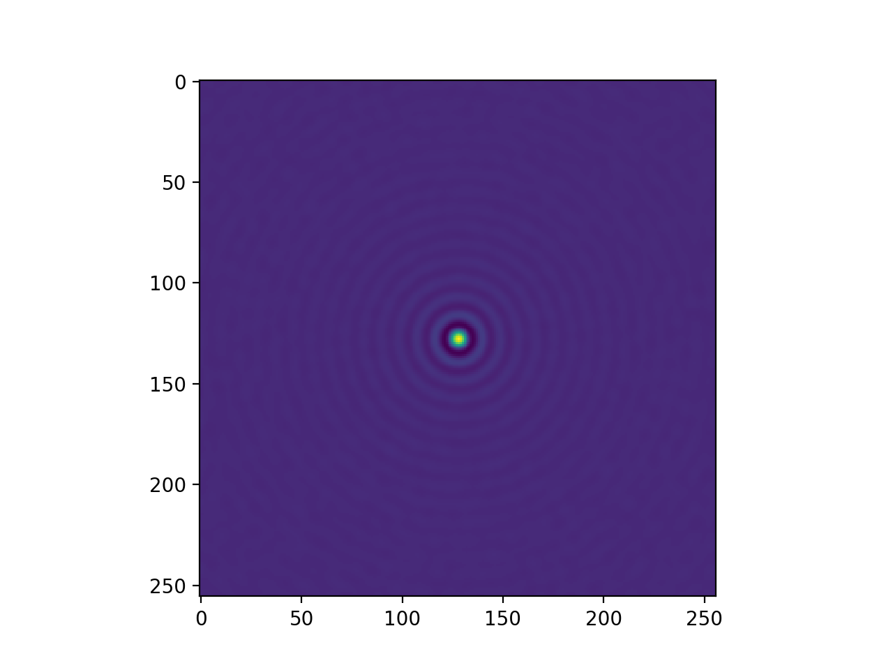
An example image of a point source, generated using a filled aperture and plotted using matplotlib.

__init__(precision=None, settings=None)¶

Creates an OSKAR imager.

Parameters:	precision (Optional[str]) – Either ‘double’ or ‘single’ to specify the numerical precision of the images. Default ‘double’. settings (Optional[oskar.SettingsTree]) – Optional settings to use to set up the imager.

algorithm¶

Returns or sets the algorithm used by the imager. Currently one of ‘FFT’, ‘DFT 2D’, ‘DFT 3D’ or ‘W-projection’.

The default is ‘FFT’, which corresponds to basic but quick 2D gridding, ignoring baseline w-components. DFT-based methods are (very, very!) slow but more accurate. The ‘DFT 3D’ option can be used to make a “perfect” undistorted dirty image, but should only be considered for use with small data sets.

Use ‘W-projection’ (or your favourite other imaging tool - there are many!) to avoid distortions caused by imaging wide fields of view using non-coplanar baselines. The implementation of W-projection in OSKAR produces results consistent with dirty images from CASA, although the GPU version in OSKAR is considerably faster for large visibility data sets: use grid_on_gpu (and optionally fft_on_gpu) to enable it, but ensure you have enough GPU memory available for the size of image you are making, as an extra copy of the grid will be made by the FFT library.

Type: str

cellsize_arcsec¶

Returns or sets the cell (pixel) size, in arcsec.

After setting this property, changing the image size will change the field of view. Can be used instead of fov_deg if required.

Type: float

channel_snapshots¶

Returns or sets the flag to image channels separately.

By default, this is false.

Type: boolean

coords_only¶

Returns or sets the flag to use coordinates only.

Set this property when using uniform weighting or W-projection. The grids of weights can only be used once they are fully populated, so this method puts the imager into a mode where it only updates its internal weights grids when calling update().

This should only be used after setting all imager options.

Turn this mode off when processing visibilities, otherwise they will be ignored.

Type: boolean

fft_on_gpu¶

Returns or sets the flag to use the GPU for FFTs.

By default, this is false.

Type: boolean

fov_deg¶

Returns or sets the image field-of-view, in degrees.

After setting this property, changing the image size will change the image resolution. Can be used instead of cellsize_arcsec if required.

Type: float

freq_max_hz¶

Returns or sets the maximum frequency of visibility data to image.

A value less than or equal to zero means no maximum.

Type: float

freq_min_hz¶

Returns or sets the minimum frequency of visibility data to image.

Type: float

generate_w_kernels_on_gpu¶

Returns or sets the flag to use the GPU to generate kernels for W-projection.

By default, this is true.

Type: boolean

grid_on_gpu¶

Returns or sets the flag to use the GPU for gridding.

By default, this is false.

Type: boolean

image_size¶

Returns or sets the image side length in pixels.

Type: int

image_type¶

Returns or sets the image (polarisation) type.

Either ‘STOKES’, ‘I’, ‘Q’, ‘U’, ‘V’, ‘LINEAR’, ‘XX’, ‘XY’, ‘YX’, ‘YY’ or ‘PSF’.

By default, this is ‘I’ (for Stokes I only).

Type: str

input_file¶

Returns or sets the input visibility file or Measurement Set.

Type: str

ms_column¶

Returns or sets the data column to use from a Measurement Set.

Type: str

num_w_planes¶

Returns or sets the number of W-projection planes to use, if using W-projection.

A number less than or equal to zero means ‘automatic’.

Type: int

output_root¶

Returns or sets the root path of output images.

Type: str

plane_size¶

Returns the required plane side length.

This may be different to the image size, for example if using W-projection. It will only be valid after a call to check_init().

Type: int

root_path¶

Returns or sets the root path of output images.

Type: str

scale_norm_with_num_input_files¶

Returns or sets the option to scale image normalisation with the number of files.

Set this to true if the different files represent multiple sky model components observed with the same telescope configuration and observation parameters. Set this to false if the different files represent multiple observations of the same sky with different telescope configurations or observation parameters.

By default, this is false.

Type: boolean

size¶

Returns or sets the image side length in pixels.

Type: int

time_max_utc¶

Returns or sets the maximum time of visibility data to image.

A value less than or equal to zero means no maximum. The value is given as MJD(UTC).

Type: float

time_min_utc¶

Returns or sets the minimum time of visibility data to image.

The value is given as MJD(UTC).

Type: float

uv_filter_max¶

Returns or sets the maximum UV baseline length to image, in wavelengths.

A value less than zero means no maximum (i.e. all baseline lengths are allowed).

Type: float

uv_filter_min¶

Returns or sets the minimum UV baseline length to image, in wavelengths.

Type: float

weighting¶

Returns or sets the type of visibility weighting to use.

Either ‘Natural’, ‘Radial’ or ‘Uniform’. The default is ‘Natural’.

Type: str

wprojplanes¶

Returns or sets the number of W-projection planes to use, if using W-projection.

A number less than or equal to zero means ‘automatic’.

Type: int

check_init()¶

Initialises the imager algorithm if it has not already been done.

All imager options and data must have been set appropriately before calling this function.

finalise(return_images=0, return_grids=0)¶

Finalises the image or images.

Images or grids can be returned in a Python dictionary of numpy arrays, if required. The image cube can be accessed using the ‘images’ key, and the grid cube can be accessed using the ‘grids’ key. Use e.g. [‘images’][0] to access the first image.

Parameters:	return_images (Optional[int]) – Number of image planes to return. return_grids (Optional[int]) – Number of grid planes to return.
Returns:	Python dictionary containing two keys, ‘images’ and ‘grids’, which are themselves arrays.
Return type:	dict

finalise_plane(plane, plane_norm)¶

Finalises an image plane.

This is a low-level function that is used to finalise gridded visibilities when used in conjunction with update_plane().

The image can be obtained by taking the real part of the plane after this function returns.

Parameters:	plane (complex float, array-like) – On input, the plane to finalise; on output, the image plane. plane_norm (float) – Plane normalisation to apply.

reset_cache()¶

Low-level function to reset the imager’s internal memory.

This is used to clear any data added using update().

rotate_coords(uu_in, vv_in, ww_in)¶

Rotates baseline coordinates to the new phase centre (if set).

Prior to calling this method, the new phase centre must be set first using set_direction(), and then the original phase centre must be set using set_vis_phase_centre(). Note that the order of these calls is important.

Parameters:	uu_in (numpy.ndarray) – Baseline uu coordinates. vv_in (numpy.ndarray) – Baseline vv coordinates. ww_in (numpy.ndarray) – Baseline ww coordinates.

rotate_vis(uu_in, vv_in, ww_in, vis)¶

Phase-rotates visibility amplitudes to the new phase centre (if set).

Prior to calling this method, the new phase centre must be set first using set_direction(), and then the original phase centre must be set using set_vis_phase_centre(). Note that the order of these calls is important.

Note that the coordinates (uu_in, vv_in, ww_in) correspond to the original phase centre, and must be in wavelengths.

Parameters:	uu_in (float, array-like) – Original baseline uu coordinates, in wavelengths. vv_in (float, array-like) – Original baseline vv coordinates, in wavelengths. ww_in (float, array-like) – Original baseline ww coordinates, in wavelengths. vis (numpy.ndarray) – Complex visibility amplitudes.

run(uu=None, vv=None, ww=None, amps=None, weight=None, time_centroid=None, start_channel=0, end_channel=0, num_pols=1, return_images=0, return_grids=0)¶

Runs the imager.

Visibilities will be used either from the input file or Measurement Set, if one is set, or from the supplied arrays. If using a file, the input filename must be set using input_file. If using arrays, the visibility meta-data must be set prior to calling this method using set_vis_frequency() and set_vis_phase_centre().

The visibility amplitude data dimension order must be: (slowest) time/baseline, channel, polarisation (fastest). This order is the same as that stored in a Measurement Set.

The visibility weight data dimension order must be: (slowest) time/baseline, polarisation (fastest).

If not given, the weights will be treated as all 1.

Images or grids can be returned in a Python dictionary of numpy arrays, if required. The image cube can be accessed using the ‘images’ key, and the grid cube can be accessed using the ‘grids’ key. Use e.g. [‘images’][0] to access the first image.

Parameters:	uu (Optional[float, array-like, shape (n,)]) – Time-baseline ordered uu coordinates, in metres. vv (Optional[float, array-like, shape (n,)]) – Time-baseline ordered vv coordinates, in metres. ww (Optional[float, array-like, shape (n,)]) – Time-baseline ordered ww coordinates, in metres. amps (Optional[complex float, array-like, shape (m,)]) – Baseline visibility amplitudes. Length as described above. weight (Optional[float, array-like, shape (p,)]) – Visibility weights. Length as described above. time_centroid (Optional[float, array-like, shape (n,)]) – Visibility time centroid values, as MJD(UTC) seconds. start_channel (Optional[int]) – Start channel index of the visibility block. Default 0. end_channel (Optional[int]) – End channel index of the visibility block. Default 0. num_pols (Optional[int]) – Number of polarisations in the visibility block. Default 1. return_images (Optional[int]) – Number of image planes to return. return_grids (Optional[int]) – Number of grid planes to return.
Returns:	Python dictionary containing two keys, ‘images’ and ‘grids’, which are themselves arrays.
Return type:	dict

set(**kwargs)¶

Sets multiple properties at once.

Example: set(fov_deg=2.0, image_size=2048, algorithm=’W-projection’)

set_default_direction()¶: Clears any direction override.

set_direction(ra_deg, dec_deg)¶

Sets the image centre different to the observation phase centre.

Parameters:	ra_deg (float) – The new image Right Ascension, in degrees. dec_deg (float) – The new image Declination, in degrees.

set_grid_kernel(kernel_type, support, oversample)¶

Sets the convolution kernel used for gridding visibilities.

Parameters:	kernel_type (str) – Type of convolution kernel; either ‘Spheroidal’ or ‘Pillbox’. support (int) – Support size of kernel. The kernel width is 2 * support + 1. oversample (int) – Oversample factor used for look-up table.

set_vis_frequency(ref_hz, inc_hz=0.0, num_channels=1)¶

Sets the visibility start frequency.

Parameters:	ref_hz (float) – Frequency of channel index 0, in Hz. inc_hz (Optional[float]) – Frequency increment, in Hz. Default 0.0. num_channels (Optional[int]) – Number of channels in visibility data. Default 1.

set_vis_phase_centre(ra_deg, dec_deg)¶

Sets the coordinates of the visibility phase centre.

Parameters:	ra_deg (float) – Right Ascension of phase centre, in degrees. dec_deg (float) – Declination of phase centre, in degrees.

update(uu, vv, ww, amps=None, weight=None, time_centroid=None, start_channel=0, end_channel=0, num_pols=1)¶

Runs imager for supplied visibilities, applying optional selection.

The visibility meta-data must be set prior to calling this method using set_vis_frequency() and set_vis_phase_centre().

The visibility amplitude data dimension order must be: (slowest) time/baseline, channel, polarisation (fastest). This order is the same as that stored in a Measurement Set.

The visibility weight data dimension order must be: (slowest) time/baseline, polarisation (fastest).

If not given, the weights will be treated as all 1.

The time_centroid parameter may be None if time filtering is not required.

Call finalise() to finalise the images after calling this function.

Parameters:

uu (float, array-like, shape (n,)) – Visibility uu coordinates, in metres.
vv (float, array-like, shape (n,)) – Visibility vv coordinates, in metres.
ww (float, array-like, shape (n,)) – Visibility ww coordinates, in metres.
amps (Optional[complex float, array-like, shape (m,)]) – Visibility complex amplitudes. Shape as described above.
weight (Optional[float, array-like, shape (p,)]) – Visibility weights. Shape as described above.
time_centroid (Optional[float, array-like, shape (n,)]) – Visibility time centroid values, as MJD(UTC) seconds.
start_channel (Optional[int]) – Start channel index of the visibility block. Default 0.
end_channel (Optional[int]) – End channel index of the visibility block. Default 0.
num_pols (Optional[int]) – Number of polarisations in the visibility block. Default 1.

update_from_block(header, block)¶

Runs imager for visibility block, applying optional selection.

Call finalise() to finalise the images after calling this function.

Parameters:	header (oskar.VisHeader) – OSKAR visibility header. block (oskar.VisBlock) – OSKAR visibility block.

update_plane(uu, vv, ww, amps, weight, plane, plane_norm, weights_grid=None)¶

Updates the supplied plane with the supplied visibilities.

This is a low-level function that can be used to generate gridded visibilities if required.

Visibility selection/filtering and phase rotation are not available at this level.

When using a DFT, plane refers to the image plane; otherwise, plane refers to the visibility grid.

The supplied baseline coordinates must be in wavelengths.

If this is called in “coordinate only” mode, then the visibility amplitudes are ignored, the plane is untouched and the weights grid is updated instead.

If the weight parameter is None, the weights will be treated as all 1.

Call finalise_plane() to finalise the image after calling this function.

Parameters:	uu (float, array-like, shape (n,)) – Visibility uu coordinates, in wavelengths. vv (float, array-like, shape (n,)) – Visibility vv coordinates, in wavelengths. ww (float, array-like, shape (n,)) – Visibility ww coordinates, in wavelengths. amps (complex float, array-like, shape (n,) or None) – Visibility complex amplitudes. weight (float, array-like, shape (n,) or None) – Visibility weights. plane (float, array-like or None) – Plane to update. plane_norm (float) – Current plane normalisation. weights_grid (Optional[float, array-like]) – Gridded weights, size and shape of the grid plane. Used for uniform weighting.
Returns:	Updated plane normalisation.
Return type:	float

static cellsize_to_fov(cellsize_rad, size)¶

Convert image cellsize and size along one dimension in pixels to FoV.

Parameters:	cellsize_rad (float) – Image cell size, in radians. size (int) – Image size in one dimension in pixels.
Returns:	Image field-of-view, in radians.
Return type:	float

static fov_to_cellsize(fov_rad, size)¶

Convert image FoV and size along one dimension in pixels to cellsize.

Parameters:	fov_rad (float) – Image field-of-view, in radians. size (int) – Image size in one dimension in pixels.
Returns:	Image cellsize, in radians.
Return type:	float

static fov_to_uv_cellsize(fov_rad, size)¶

Convert image FoV and size along one dimension in pixels to cellsize.

Parameters:	fov_rad (float) – Image field-of-view, in radians. size (int) – Image size in one dimension in pixels.
Returns:	UV cellsize, in wavelengths.
Return type:	float

static uv_cellsize_to_fov(uv_cellsize, size)¶

Convert a uv cellsize in wavelengths to an image FoV, in radians.

uv cellsize is the size of a uv grid pixel in the grid used when imaging using an FFT.

Parameters:	uv_cellsize (float) – Grid pixel size in wavelengths size (int) – Size of the uv grid in pixels.
Returns:	Image field-of-view, in radians
Return type:	float

static extent_pixels(size)¶

Obtain the image or grid extent in pixel space

Parameters:	size (int) – Image or grid size (number of pixels)
Returns:	Image or grid extent in pixels ordered as follows [x_min, x_max, y_min, y_max]
Return type:	numpy.ndarray

static image_extent_lm(fov_deg, size)¶

Return the image extent in direction cosines.

The image extent is a list of 4 elements describing the dimensions of the image in the x (l) and y (m) axes. This can be used for example, to label images produced using the OSKAR imager when plotted with matplotlib’s imshow() method.

Parameters:	fov_deg (float) – Image field-of-view, in degrees size (int) – Image size (number of pixels)
Returns:	Image extent in direction cosines ordered as follows [l_min, l_max, m_min, m_max]
Return type:	numpy.ndarray

static grid_extent_wavelengths(fov_deg, size)¶

Return the the uv grid extent in wavelengths.

The grid extent is a list of 4 elements describing the dimensions of the uv grid in the x (uu) and y (vv) axes. This can be used for example, to label uv grid images produced using the OSKAR imager when plotted with matplotlib’s imshow() method.

Parameters:	fov_deg (float) – Image field-of-view, in degrees size (int) – Grid / image size (number of pixels)
Returns:	Grid extent in wavelengths ordered as follows [uu_min, uu_max, vv_min, vv_max]
Return type:	numpy.ndarray

static grid_pixels(grid_cellsize, size)¶

Return grid pixel coordinates the same units as grid_cellsize.

Returns the x and y coordinates of the uv grid pixels for a grid / image of size x size pixels where the grid pixel separation is given by grid_cellsize. The output pixel coordinates will be in the same units as that of the supplied grid_cellsize.

Parameters:	grid_cellsize (float) – Pixel separation in the grid size (int) – Size of the grid / image
Returns:	The tuple elements gx and gy are the pixel coordinates of each grid cell. gx and gy are 2D arrays of dimensions size by size.
Return type:	tuple

static image_pixels(fov_deg, im_size)¶

Return image pixel coordinates in lm (direction cosine) space.

Parameters:	fov_deg – Image field-of-view in degrees im_size – Image size in pixels.
Returns:	The tuple elements l and m are the coordinates of each image pixel in the l (x) and m (y) directions. l and m are 2D arrays of dimensions im_size by im_size
Return type:	tuple

static make_image(uu, vv, ww, amps, fov_deg, size, weighting='Natural', algorithm='FFT', weight=None, wprojplanes=0)¶

Makes an image from visibility data.

Convenience static function.

Parameters:	uu (float, array-like, shape (n,)) – Baseline uu coordinates, in wavelengths. vv (float, array-like, shape (n,)) – Baseline vv coordinates, in wavelengths. ww (float, array-like, shape (n,)) – Baseline ww coordinates, in wavelengths. amps (complex float, array-like, shape (n,)) – Baseline visibility amplitudes. fov_deg (float) – Image field of view, in degrees. size (int) – Image size along one dimension, in pixels. weighting (Optional[str]) – Either ‘Natural’, ‘Radial’ or ‘Uniform’. algorithm (Optional[str]) – Algorithm type: ‘FFT’, ‘DFT 2D’, ‘DFT 3D’ or ‘W-projection’. weight (Optional[float, array-like, shape (n,)]) – Visibility weights. wprojplanes (Optional[int]) – Number of W-projection planes to use, if using W-projection. If <= 0, this will be determined automatically. It will not be less than 16.
Returns:	Image as a 2D numpy array. Data are ordered as in FITS image.
Return type:	numpy.ndarray