Simple “hello world” example
This is a simple “hello world”-style simulation and imaging example
to show basic usage of the main OSKAR Python classes. It can be run
interactively from either an ipython prompt or a Jupyter notebook,
or as a complete Python script (which is given at the bottom of the page).
Note
This example uses the telescope model from the OSKAR example data, so make sure this is unpacked into the directory from which this script is run.
We require the matplotlib, numpy and oskar Python modules.
The sky model will be created from a numpy array, and we will use
matplotlib to render the output image as a PNG file.
import matplotlib
matplotlib.use("Agg")
import matplotlib.pyplot as plt
import numpy
import oskar
First we set up a oskar.SettingsTree from a Python dictionary.
Note that not all settings are defined at this stage.
As the sky model will be very small for this example, we choose not to
use GPUs here, hence simulator/use_gpus is set to false.
params = {
    "simulator": {
        "use_gpus": False
    },
    "observation" : {
        "num_channels": 3,
        "start_frequency_hz": 100e6,
        "frequency_inc_hz": 20e6,
        "phase_centre_ra_deg": 20,
        "phase_centre_dec_deg": -30,
        "num_time_steps": 24,
        "start_time_utc": "01-01-2000 12:00:00.000",
        "length": "12:00:00.000"
    },
    "telescope": {
        "input_directory": "telescope.tm"
    },
    "interferometer": {
        "oskar_vis_filename": "example.vis",
        "ms_filename": "",
        "channel_bandwidth_hz": 1e6,
        "time_average_sec": 10
    }
}
settings = oskar.SettingsTree("oskar_sim_interferometer")
settings.from_dict(params)
We choose the numerical precision to use (single or double) when
running the simulation, and update one of the settings accordingly.
precision = "single"
if precision == "single":
    settings["simulator/double_precision"] = False
The sky model will contain only three sources, which are stored in a
numpy array. The sky model is created with the appropriate precision
using oskar.Sky.from_array().
sky_data = numpy.array([
        [20.0, -30.0, 1, 0, 0, 0, 100.0e6, -0.7, 0.0, 0,   0,   0],
        [20.0, -30.5, 3, 2, 2, 0, 100.0e6, -0.7, 0.0, 600, 50,  45],
        [20.5, -30.5, 3, 0, 0, 2, 100.0e6, -0.7, 0.0, 700, 10, -10]])
sky = oskar.Sky.from_array(sky_data, precision)  # Pass precision here.
Next, we create the oskar.Interferometer simulator, set the sky model
and run the simulation to generate visibilities.
Visibility data will be saved to a binary data file named example.vis.
(To save it in the CASA Measurement Set format, specify a value for
the interferometer/ms_filename parameter in the settings tree.)
sim = oskar.Interferometer(settings=settings)
sim.set_sky_model(sky)
sim.run()
The simulated visibilities can now be imaged using oskar.Imager.
This example uses the set() method to set
multiple properties using the same call. This image will only be 512 pixels
across and will have a field of view of 4 degrees.
A FITS file named example_I.fits will also be written.
The image is returned to Python and can be accessed from the dictionary
of arrays returned by oskar.Imager.run().
imager = oskar.Imager(precision)
imager.set(fov_deg=4, image_size=512)
imager.set(input_file="example.vis", output_root="example")
output = imager.run(return_images=1)
image = output["images"][0]
Finally, the image is plotted using matplotlib and saved as a PNG file
called example.png, which is included below.
im = plt.imshow(image, cmap="jet")
plt.gca().invert_yaxis()
plt.colorbar(im)
plt.savefig("%s.png" % imager.output_root)
plt.close("all")
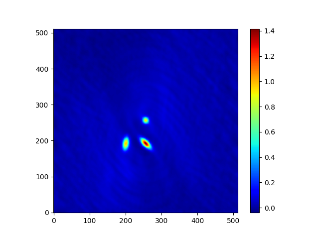
An example image generated using OSKAR and plotted using matplotlib
For completeness, the whole script is available here
(hello-world.py):
#!/usr/bin/env python3

"""Script to run a simple test example of an OSKAR simulation."""

import matplotlib
matplotlib.use("Agg")
# pylint: disable=wrong-import-position
import matplotlib.pyplot as plt
import numpy
import oskar

# Basic settings. (Note that the sky model is set up later.)
params = {
    "simulator": {
        "use_gpus": False
    },
    "observation" : {
        "num_channels": 3,
        "start_frequency_hz": 100e6,
        "frequency_inc_hz": 20e6,
        "phase_centre_ra_deg": 20,
        "phase_centre_dec_deg": -30,
        "num_time_steps": 24,
        "start_time_utc": "01-01-2000 12:00:00.000",
        "length": "12:00:00.000"
    },
    "telescope": {
        "input_directory": "telescope.tm"
    },
    "interferometer": {
        "oskar_vis_filename": "example.vis",
        "ms_filename": "",
        "channel_bandwidth_hz": 1e6,
        "time_average_sec": 10
    }
}
settings = oskar.SettingsTree("oskar_sim_interferometer")
settings.from_dict(params)

# Set the numerical precision to use.
precision = "single"
if precision == "single":
    settings["simulator/double_precision"] = False

# Create a sky model containing three sources from a numpy array.
sky_data = numpy.array([
        [20.0, -30.0, 1, 0, 0, 0, 100.0e6, -0.7, 0.0, 0,   0,   0],
        [20.0, -30.5, 3, 2, 2, 0, 100.0e6, -0.7, 0.0, 600, 50,  45],
        [20.5, -30.5, 3, 0, 0, 2, 100.0e6, -0.7, 0.0, 700, 10, -10]])
sky = oskar.Sky.from_array(sky_data, precision)  # Pass precision here.

# Set the sky model and run the simulation.
sim = oskar.Interferometer(settings=settings)
sim.set_sky_model(sky)
sim.run()

# Make an image 4 degrees across and return it to Python.
# (It will also be saved with the filename "example_I.fits".)
imager = oskar.Imager(precision)
imager.set(fov_deg=4, image_size=512)
imager.set(input_file="example.vis", output_root="example")
output = imager.run(return_images=1)
image = output["images"][0]

# Render the image using matplotlib and save it as a PNG file.
im = plt.imshow(image, cmap="jet")
plt.gca().invert_yaxis()
plt.colorbar(im)
plt.savefig("%s.png" % imager.output_root)
plt.close("all")